AN-004 · application note · quant
Bitcoin Regime Analysis, Part 2: What Each Feature Buys You
Volatility buys long regimes with no direction. Volume buys direction but halves regime length. Fractional differencing buys length back and destroys direction completely. Every one of those is a trade, not an improvement.
- published
- length
- 11 min·2,295 words
- application
- quant/research
- terms
- cryptocurrency, bitcoin, regime-analysis, hidden-markov-model, time-series
Part 1 established that Bitcoin’s hourly returns have almost no linear predictability, strongly clustered volatility, fat tails, and long memory in the variance but not the mean. That is close to a description of what a regime-switching model assumes, so this post fits some.
The plan is to start with the simplest specification and add one feature at a time: returns alone, then volatility, then volume, then a different way of preparing the returns. The interesting part isn’t which model wins. It’s that every feature turned out to be a trade rather than an improvement — each one bought something and cost something else.
Same scope as Part 1: I’m characterising what these models find, not building or testing a trading signal. Nothing is validated out of sample and no returns are claimed.
One more thing, up front. I re-ran everything from scratch to write this up, and that turned up a genuine bug in my own feature construction plus a much bigger seed-sensitivity problem than I expected. Both are in here, because both changed the conclusions.
§What the model is actually doing
If you’ve used HMMs in NLP, this is the same machinery with different nouns.
You assume a hidden state you never observe directly. At each step the system sits in one of K states, and the state determines the distribution your observation is drawn from. States tend to persist, and you infer the sequence of hidden states from the observations they produced.
In NLP the hidden state might be a grammatical context and the observation a word. Here the state is a market regime and the observation is an hourly return.
I’m using a Gaussian HMM with diagonal covariance, so each state gets its own mean and variance in every feature it’s handed, but no cross-feature correlation. That matters for everything below: each feature you add is an independent axis a state can be told apart on, and nothing else.
Two notes on reading the charts. Labels come from Viterbi decoding, which picks the most likely sequence of states rather than scoring each bar alone, so a label is informed by its neighbours. I fit and decode in independent 24-hour blocks, which bounds that to at most 23 hours of context inside the same day rather than the whole 18-month series. And all of it is in-sample.
§Attempt 1: returns only
One feature — the log-return — and three states.
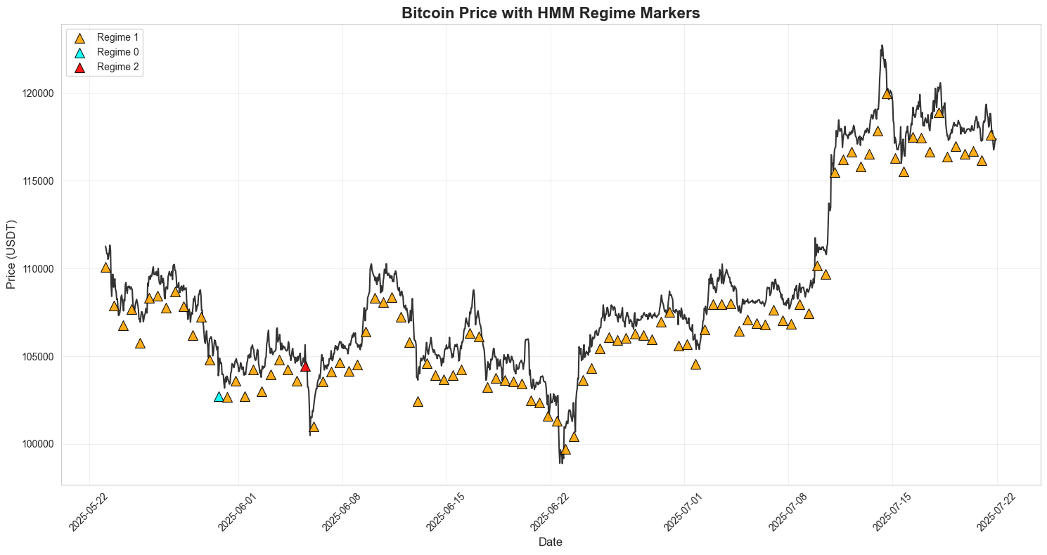
Figure 1: Three states, returns only
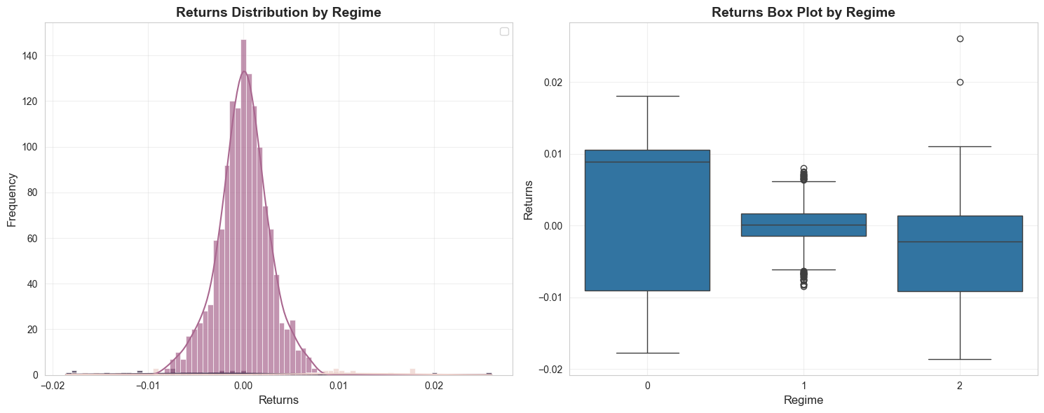
Figure 2: One tight distribution near zero, two wider ones
| state | share | mean return | std dev |
|---|---|---|---|
| 1 | 84.1% | 9.20 × 10⁻⁵ | 3.15 × 10⁻³ |
| 2 | 11.6% | −4.02 × 10⁻⁴ | 1.15 × 10⁻² |
| 0 | 4.3% | 6.18 × 10⁻⁴ | 7.85 × 10⁻³ |
A calm state covering most of the series, and two volatile ones differing by size. The model has rediscovered volatility, which makes sense: given only returns, the main thing states can differ in is spread.
§Now ask for five states
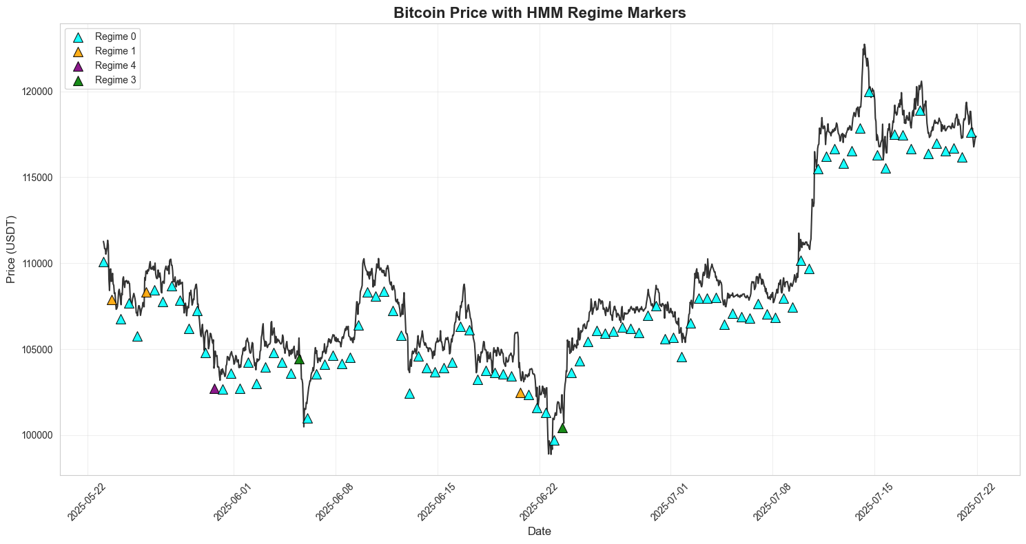
Figure 3: Five states, returns only
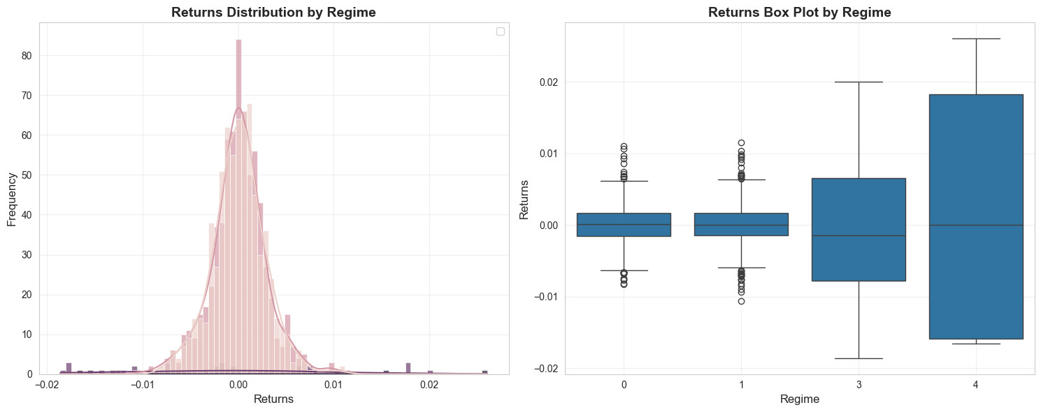
Figure 4: Regimes 0 and 1 are indistinguishable — and Regime 2 is missing from the boxplot entirely
| state | share | mean return | std dev |
|---|---|---|---|
| 1 | 42.7% | 1.70 × 10⁻⁴ | 3.59 × 10⁻³ |
| 0 | 41.9% | 4.99 × 10⁻⁵ | 3.46 × 10⁻³ |
| 3 | 14.3% | −4.84 × 10⁻⁵ | 9.22 × 10⁻³ |
| 4 | 0.7% | 1.09 × 10⁻³ | 1.40 × 10⁻² |
| 2 | 0.4% | −2.72 × 10⁻³ | 2.43 × 10⁻² |
States 0 and 1 differ in mean by 0.03 standard deviations and in spread by 3.8%. They are one state fitted twice, and together they cover 84.6% — almost exactly the 84.1% the single calm state held at K=3. The model took the calm regime and sawed it in half. State 2 got 0.4% of the data, which is why it never appears in the boxplot.
This is the lesson the rest of the post is built on. The model isn’t struggling because it needs better initialisation. There is only one dimension along which states can differ, and with a single feature a state is fully described by a mean and a variance. You run out of distinguishable shapes at three or four, and after that the optimiser splits a state and hands you a duplicate.
§The criteria agree, and so does the clock
| K | AIC | BIC | state switches | mean regime duration |
|---|---|---|---|---|
| 2 | −102,840 | −102,788 | 697 | 11.4 h |
| 3 | −102,913 | −102,809 | 1,338 | 4.8 h |
| 4 | −103,095 | −102,923 | 772 | 6.0 h |
| 5 | −102,761 | −102,507 | 11,166 | 2.3 h |
| 6 | −102,636 | −102,285 | 12,521 | 1.3 h |
| 7 | −102,427 | −101,964 | 12,870 | 1.0 h |
Both criteria bottom out at K = 4. But the switch count is what lands: the series has 12,888 hourly observations, so at K=7 the model changes state 12,870 times — 99.9% of bars. A regime that lasts one hour is a relabelling of the return itself.
§Attempt 2: add volatility
The first new axis is a volatility estimate from FIGARCH(1,1) with Student-t innovations, refitted on a rolling one-week (168-hour) window as a one-step-ahead forecast.
FIGARCH lets volatility shocks persist far longer than ordinary GARCH, which is what Part 1’s Hurst exponent of 0.6–0.9 on volatility was describing. The Student-t is deliberate: Part 1 measured excess kurtosis of 9.44, and a Gaussian likelihood would understate exactly the moves that matter. And because each estimate is forecast one step ahead from a trailing window, the volatility feature only ever sees the past.
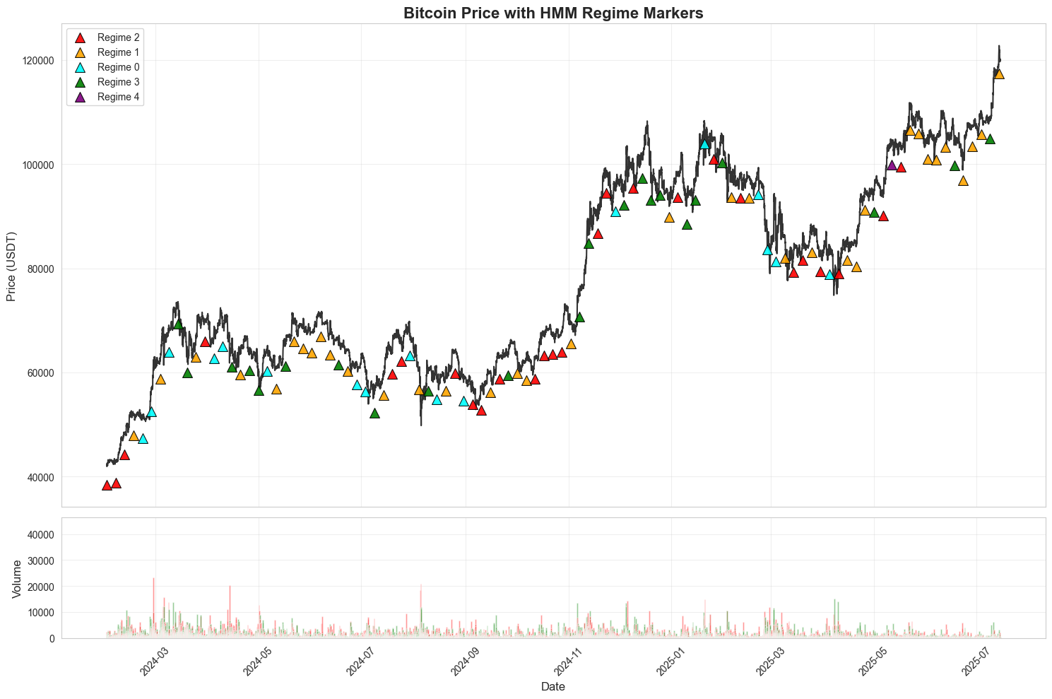
Figure 5: Five states, returns plus volatility
The degeneracy is gone, and regimes get dramatically longer:
| K | BIC | switches | mean duration |
|---|---|---|---|
| 3 | −1,018 | 6.1% | 17.4 h |
| 5 | −7,695 | 11.8% | 9.6 h |
| 6 | −9,166 | 16.0% | 8.0 h |
| 7 | −9,491 | 17.4% | 6.0 h |
Seven states switching on 17% of bars with a six-hour average life, against 99.9% and one hour for returns alone. That is a real gain.
But it buys no direction whatsoever. Across six random seeds at K=7, the gap between the most bullish and most bearish state’s mean return has a median of 0.118, and never once exceeds 0.3. Volatility sorts periods by how violent they are while staying completely agnostic about which way they went. Every state is, on average, flat.
§Attempt 3: add volume
Volume contributes something neither of the others can: how many people are involved.
The feature isn’t raw volume, and isn’t quite relative volume either. It’s |return| × RVOL, standardised — where RVOL is volume over its own 24-hour rolling mean. It’s high when a large move coincides with unusually heavy participation. It measures conviction rather than activity.
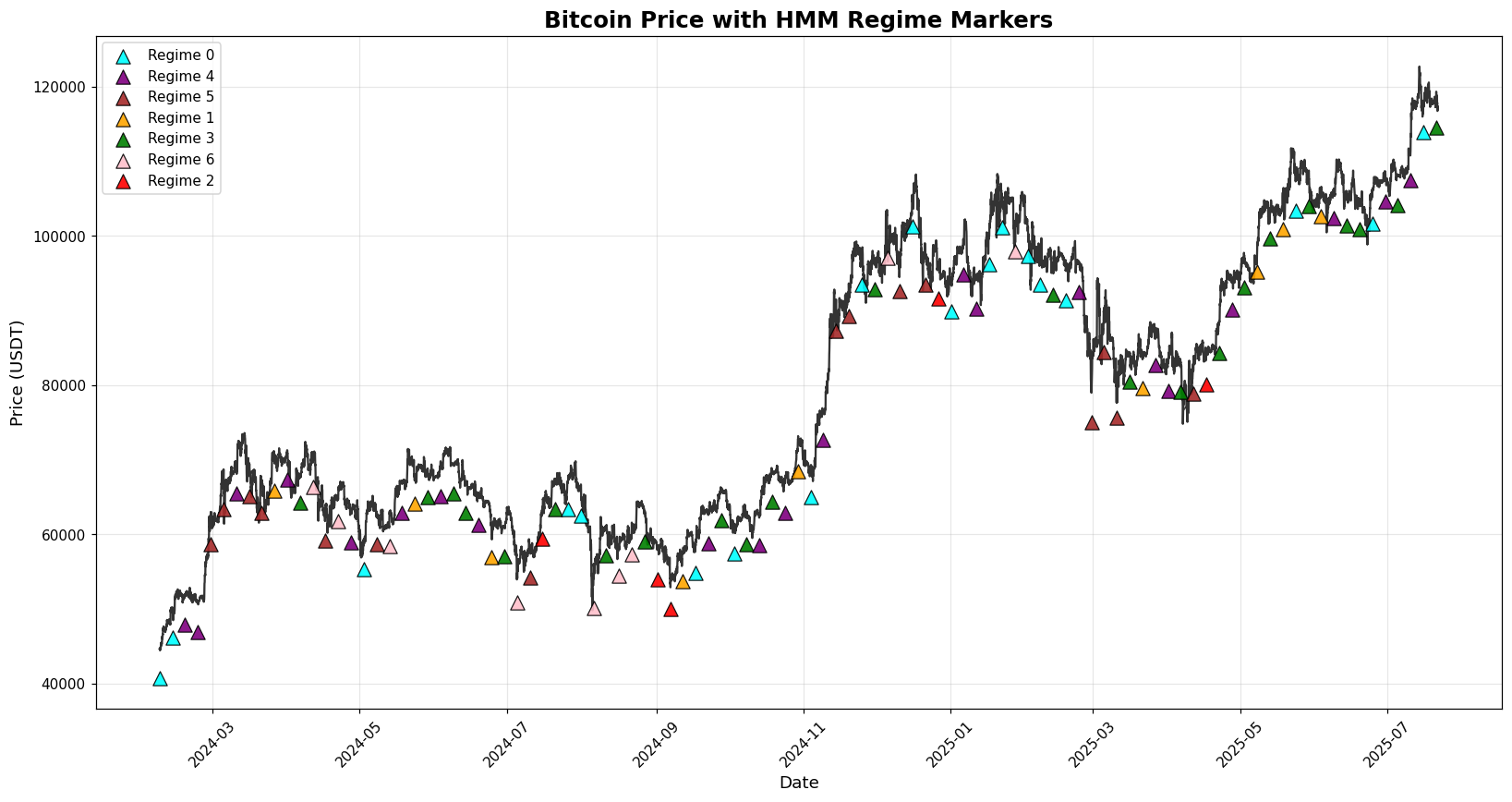
Figure 6: Seven states with returns, volatility and volume (seed 0 — see the seed table below)
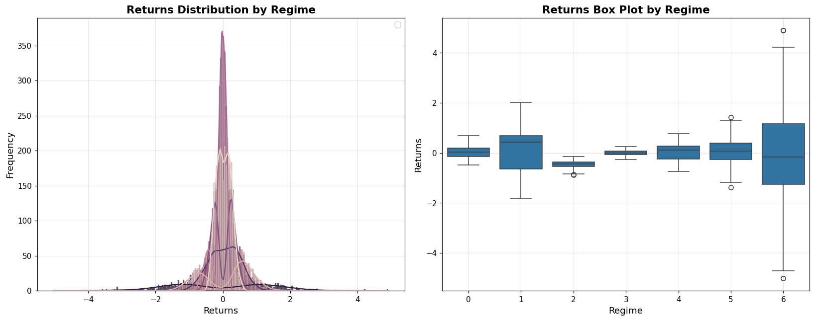
Figure 7: Regime 2 sits clearly below zero; Regime 6 is the wide, heavy-volume stress state
| state | share | mean return | sd return | mean |r|×RVOL |
|---|---|---|---|---|
| 2 | 4.1% | −0.454 | 0.138 | −0.065 |
| 6 | 6.9% | −0.067 | 1.519 | +2.125 |
| 3 | 20.4% | −0.002 | 0.098 | −0.354 |
| 4 | 16.6% | +0.014 | 0.300 | −0.189 |
| 0 | 25.5% | +0.032 | 0.214 | −0.304 |
| 5 | 15.9% | +0.056 | 0.441 | −0.141 |
| 1 | 10.7% | +0.103 | 0.736 | +0.468 |
Two things appear that weren’t there before.
Direction. State 2 has a mean return of −0.454, an order of magnitude beyond anything the volatility-only model produced. Across six seeds the directional spread has a median of 0.665 and clears 0.3 in five of six runs, against a median of 0.118 and zero of six without volume. That’s a 5.7× increase, and unlike a single fit it’s a claim about the distribution of fits rather than one lucky draw.
A stress state. State 6 carries a volume-interaction of +2.13 — four and a half times any other state — alongside by far the widest returns. Big moves on heavy participation, which is the capitulation signature.
And it costs something. Mean regime duration falls from 6.1 hours to 2.2 hours, and switching rises from 17% of bars to 45%. Volume buys direction by paying in persistence.
§Attempt 4: fractional differentiation
The last change isn’t a new feature. It’s a different way of preparing the returns.
Raw prices carry memory but aren’t stationary. Difference them once and you get returns: stationary, but nearly all the memory is gone. Fractional differentiation (López de Prado, 2018) makes the choice continuous — difference by a fractional amount, here d = 0.3 on log price, keeping more memory than a full difference would.
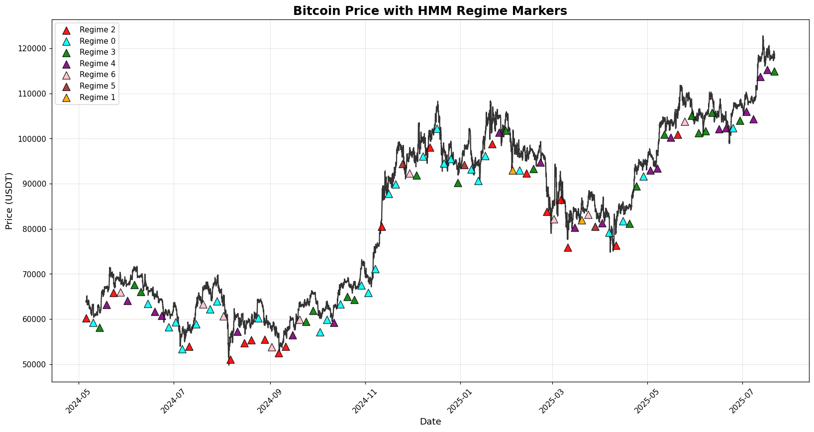
Figure 8: Seven states with fractionally differenced returns (seed 0)
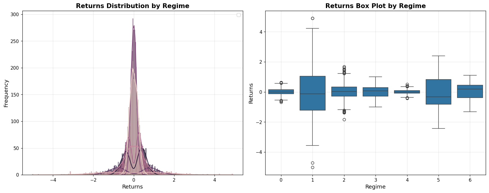
Figure 9: Every state centred at zero. They differ in spread and in nothing else.
Look at Figure 9 next to Figure 7. In the volume model one box sits clearly below zero. Here all seven sit on it.
Fractional differencing destroys directional separation completely. Across six seeds the directional spread has a median of 0.0203 — and a range of 0.018 to 0.020. That is not just small, it’s uncannily stable: every seed finds the same non-answer. The states are separating on volatility and volume, and the fractionally differenced series is close to a constant offset as far as the model is concerned.
What it does buy is persistence. Mean duration rises from 2.18 h to 2.55 h, about +17%, consistently across seeds.
So fracdiff is the mirror image of volume. Volume traded persistence for direction; fracdiff trades direction back for persistence.
§The part where I was wrong
I was originally going to report that fractional differencing produced dramatically more persistent regimes, and that the volume model found a clean symmetric bull/bear pair at ±0.58. Re-running everything killed both claims, for two different reasons.
§A three-month misalignment
Fractional differencing at d = 0.3 needs a 2,273-bar window, so the differenced series starts 2,273 hours after the raw one. My code trimmed the returns to match, then sliced the volume from the start of the series:
volume_raw = btc_df["volume"].iloc[:trimmed_length]   # starts 2024-02-01
# ...while returns and fd_returns now start 2024-05-05
The volume feature was offset from the returns by about three months. The same pattern
appears in the volume model, offset by one bar there, because diff().dropna() drops the
first observation. Both are fixed by aligning on the index instead of the position:
volume_raw = btc_df["volume"].reindex(returns.index)
With the misalignment, fractional differencing looked like it lengthened regimes by 55%. With it fixed, the honest figure is 17%.
§The bigger problem: one seed is not a result
Fixing the alignment made the ±0.58 bull/bear pair disappear entirely — at the seed I’d been using. That sent me to check how much of any of this survives a change of random seed, and the answer was humbling.
Directional spread at K=7, six seeds, volume model:
| volume feature | median | range | above 0.3 |
|---|---|---|---|
| misaligned (original) | 0.109 | 0.108 – 1.169 | 1 of 6 |
| aligned (fixed) | 0.665 | 0.091 – 1.209 | 5 of 6 |
The chart I originally published came from the misaligned data at seed 42 — which is the one seed in six where that data produces a strong directional pair. Every other seed gives about 0.11. The original figure was right for the wrong reason.
And the fixed data has the mirror-image trap: seed 42 is the one draw of six where the directional split doesn’t show up. Had I fixed the bug and kept the same seed, I’d have concluded volume does nothing.
That’s the real lesson of this post, and it isn’t about Bitcoin. A single HMM fit is a sample, not a measurement. Every claim above about direction and persistence is now a median over six seeds with the range quoted, because any one of them individually would have been capable of telling me whatever I wanted to hear.
§What each feature actually bought
All figures are medians over six seeds at K=7, with the alignment fixed:
| specification | directional spread | above 0.3 | mean duration | switching |
|---|---|---|---|---|
| returns only | n/a (degenerate) | — | 1.0 h | 99.9% |
| + volatility | 0.118 | 0 of 6 | 6.1 h | 18.7% |
| + volume | 0.665 | 5 of 6 | 2.2 h | 45.0% |
| + fractional differencing | 0.020 | 0 of 6 | 2.6 h | 38.8% |
Read across the rows and there is no “best” model, only a frontier. Volatility gives you long, stable, directionless regimes. Volume gives you direction and a capitulation state, and costs you two-thirds of your regime length. Fractional differencing gives some length back and removes direction entirely.
The through-line is still the one Figure 4 set up: an HMM can only distinguish states along dimensions you hand it. But the corollary is sharper than I expected — handing it a new dimension doesn’t just add separation, it reallocates where the separation happens. Adding volume didn’t make the model better at everything. It made it better at direction and worse at persistence, because both come out of the same likelihood.
§What this doesn’t tell you
Everything is in-sample. These describe structure found in data the model was fitted on.
Information criteria aren’t comparable across models. Each is fitted to different data on a different scale, so BIC only means something within a feature set. Returns-only is the one place criteria pick a K; elsewhere I chose K for legibility.
Six seeds is not many. It was enough to show that one seed is misleading. It is not enough to put a confidence interval on anything, and the ranges above are wide.
Regime labels aren’t stable across refits. State indices are arbitrary — “State 2” here isn’t “State 2” in the next fit. That’s why the tables are sorted by mean return rather than by index.
Identifying a regime is not the same as being able to act on one. By the time a state is clearly identifiable, much of the move it describes has happened. Nothing here addresses that, by design.
And the one I’d underline: I found a three-month misalignment in my own feature construction only because I re-ran everything to write this up, and I found the seed sensitivity only because fixing the first bug made a result vanish. Both had been sitting inside a chart I had already drawn conclusions from.